Non-parametric permutation tests or randomization tests are often recommended because they require fewer assumptions of the data. In the recent paper by Eklund et al. non-parametric permutation testing was the only method that consistently gave false positive rates in the expected range.
But how many permutations or randomizations should you perform? Answers range from “all of them” to “as many as you can” to “no more than a couple hundred”. Below I briefly describe the relationship between number of permutations performed and the confidence you can have in the resultant p-value.
When performing all possible permutations, the randomization test of \(H_0\) is guaranteed to control the probability of Type I error under the assumption of exchangeability of the randomized conditions. However, due to computational limits, enumeration of all possible permutations is not feasible in some (many) cases. Using a Monte Carlo sampling of the permutation distribution (a subset of all possible permutations), we can estimate the p value as
\[\begin{align*} \hat{p} = \frac{1 + \sum_{i=1}^{M}I(t_i \geq t^*)}{M + 1} \end{align*}\]where \(M\) is the number of permutations performed, \(t^*\) is the observed test statistic and \(t_i\) is the test statistic found on the \(i^{th}\) permutation. The Monte Carlo p value \(\hat{p}\) will vary depending on which subset of all permutations are selected. Since \(\hat{p}\) is an unbiased estimator of \(p\), we can use \(\hat{p}\) to construct a confidence interval for \(p\) based on a Normal approximation of the Binomial distribution. (Note that we could do this part non-parametrically also, but let’s not).
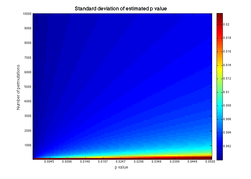
\[\begin{align} \text{standard deviation} & & s = & & \sqrt{\frac{\hat{p}(1-\hat{p})}{M}},\\ \text{confidence interval} & & (e^-,e^+) = & & (\hat{p}-zs, \hat{p}+zs) \end{align}\]where \(z\) is the critical value derived from the Normal curve and defines the level of confidence.
For example, let’s say I performed 1000 permutations and achieved a \(\hat{p}\) of 0.048 (true story). Should I reject the null hypothesis? To calculate a 95% confidence interval, I will plug in \(z = 1.96\) to the equations above, which gives the interval \([0.035, 0.061]\). For an \(\alpha\) of 0.05, I cannot reject the null hypothesis because the extreme of my confidence interval exceeds 0.05. The size of the confidence interval will increase with \(\hat{p}\) and decrease with the number of permutations. So for very small \(\hat{p}\), only few permutations are needed. But for \(\hat{p}\) near \(\alpha\), it may be impossible to perform sufficient permutations to confidently reject \(H_0\).
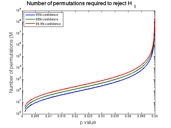
We can calculate the number of permutations required to reject \(H_0\) for a given \(\hat{p}\) by setting \(e^+ = \alpha - \epsilon\) and solving for M.
\[\begin{align*} e^+ & = \hat{p}+zs \\ & = \hat{p}+z\sqrt{\frac{\hat{p}(1-\hat{p})}{M}} = \alpha - \epsilon\\ \\ M & = \frac{\hat{p}(1-\hat{p})}{\big(\frac{\alpha - \epsilon - \hat{p}}{z}\big)^2} \end{align*}\]Thus, for the example above, if I choose \(\alpha=0.05\) and \(z=1.96\) for 95% confidence, I would need to perform 43,884 permutations in order to reject \(H_0\) with \(p=0.048\). Alternatively, had I found \(p=0.03\), I would only have needed 280 permutations.
So how many permutations should you perform? Perhaps unsatisfactorily, it does seem prudent to perform “as many as you can” to maximize the precision of your p value since you won’t know \(\hat{p}\) ahead of time. How to maximize precision while minimizing the number of required permutations appears to be an open area of research. I wonder if there could be some procedure to estimate \(\hat{p}\) with say a parametric test first, and then use that estimate to decide how many permutations to perform, but this seems akin to p-hacking somehow. In any case, we now know how to reason about the confidence of our p-values, whatever number of permutations we choose. Please comment below if you have other ideas.
References
- Ernst, M. D. (2004). Permutation Methods: A Basis for Exact Inference. Statistical Science, 19(4), 676–685. doi:10.1214/088342304000000396
- Wallis, S. (retrieved Aug 10 2016) Binomial confidence intervals and contingency tests: mathematical fundamentals and the evaluation of alternative methods
- Calculation Of The Confidence Interval (retrieved Aug 10 2016)
- Eklund, A., Nichols, T. E., & Knutsson, H. (2016). Cluster failure: Why fMRI inferences for spatial extent have inflated false-positive rates. Proceedings of the National Academy of Sciences, 113(28), 7900–7905. doi:10.1073/pnas.1602413113
- Phipson, B., and Smyth, G. K. (2010). Permutation p-values should never be zero: calculating exact p-values when permutations are randomly drawn. Stat. Appl. Genet. Molec. Biol. Volume 9, Issue 1, Article 39.
- Theo A. Knijnenburg, Lodewyk F. A. Wessels, Marcel J. T. Reinders, Ilya Shmulevich (2009) Fewer permutations, more accurate P-values. Bioinformatics. 25(12): i161–i168. doi: 10.1093/bioinformatics/btp211
Note: Thanks to Giancarlo Valente for his help with this post!